
The Myth of the Flat Line: Why Nature Never Stands Still
When students first open an ecology simulation or sketch a food web in a notebook, they almost universally expect stability to look like a straight, horizontal line. They assume that if an ecosystem has 30 rabbits and 4 wolves on Monday, a healthy habitat should still have exactly 30 rabbits and 4 wolves six months later.
Learning science research reveals that this misconception, often termed the "balance of nature myth," prevents young scientists from understanding how living systems genuinely operate. When these students see rabbit numbers decline on a telemetry chart, their immediate reaction is panic: "The ecosystem is crashing! Everything is dying!"
In living biology, a flat line does not signify health. A flat line signifies a system that is either entirely synthetic or dead. Real ecosystems exist in dynamic equilibrium: a continuous state of motion where opposing forces, such as births and deaths, consumption and replenishment, continuously push and pull against one another. Rather than resting at a static midpoint, populations naturally swing in harmonic, repeating waves.
In Level 5 of the Praxos 3D simulation ("The Dance"), we dismantle this flat-line myth. Students step onto a living meadow and observe firsthand why populations rise and fall, why wolves always lag behind rabbits, and how introducing physical hiding cover acts as a structural buffer that keeps the entire dance alive across 90 simulated days.
Ecological stability is not a frozen statue. Stability is a continuous, self-regulating wave where populations oscillate within safe upper and lower boundaries.
The Lotka-Volterra Wave: Understanding Phase Lag and Biological Delays
In the 1920s, mathematician Vito Volterra and biophysicist Alfred Lotka independently developed mathematical equations to describe the cyclical interactions between predators and their prey. Their model captures an elegant four-phase rhythmic cycle:
1. Prey Abundance Phase: When predator numbers are low and plant biomass is abundant, herbivores reproduce rapidly. The prey population curve surges upward exponentially.
2. Predator Response Phase: With abundant prey to hunt, carnivores obtain surplus calories, increasing their reproductive success and pup survival rates. Predator numbers begin to climb.
3. Over-Predation Phase: As the predator population reaches its crest, intense hunting pressure causes prey mortality to exceed births. The prey population begins a steep decline.
4. Predator Starvation Phase: With prey scarce, predators struggle to forage enough energy. Starvation increases, litters shrink, and carnivore numbers crash. With hunting pressure removed, surviving prey begin to multiply once again, restarting the cycle.
The defining feature of Lotka-Volterra dynamics is phase lag: predator peaks and troughs do not happen at the exact same instant as prey peaks and troughs. They are shifted forward in time.
This delay occurs because biological reproduction takes time. A rabbit population can spike in response to spring grass within weeks. However, wolves cannot instantaneously double their pack size overnight simply because food is abundant. Gestation periods, lactation, and pup maturation introduce an inevitable time delay into the system. In Level 5, the live graph displays a gold line for rabbits and a purple line for wolves, allowing students to observe this phase lag in real time.
| Cycle Phase | Herbivore Trend | Carnivore Trend | Underlying System Driver |
|---|---|---|---|
| SURGEPhase 1: Prey Boom | Rapid Exponential Growth | Low / Depleted Baseline | Abundant grass biomass and near-zero hunting pressure allow unconstrained breeding |
| FEEDBACKPhase 2: Predator Rise | Approaching Peak / Slowing | Rapid Upward Climb | Abundant prey calories increase carnivore litter survival after gestation delay |
| CORRECTIONPhase 3: Prey Crash | Steep Downward Decline | At Maximum Crest | High predator density exerts overwhelming predation pressure, exceeding herbivore birth rates |
| RESETPhase 4: Predator Crash | Bottoming Out / Rebounding | Steep Downward Decline | Prey scarcity causes widespread carnivore starvation, releasing pressure for the next cycle |
Real-World Evidence: The 10-Year Lynx-Hare Cycle in Boreal Forests
Is this mathematical wave just a theoretical curiosity, or does nature actually dance this way? The most famous historical demonstration of Lotka-Volterra oscillations comes from the fur-trading records of the Hudson's Bay Company in Canada. For more than a century, trappers meticulously recorded pelts collected across northern boreal forests.
When ecologists analyzed the records decades later, they uncovered an unmistakable pattern: snowshoe hare populations peaked and crashed in a rhythmic 9 to 11 year cycle. Trailing approximately one to two years behind every single hare peak was a corresponding peak in Canada lynx pelts.
When snowshoe hares multiplied across the brush, lynx flourished and raised large litters. But once millions of hares overgrazed the willow shoots and faced heavy lynx predation, the hare population collapsed. Deprived of their primary food source, lynx litters failed to survive, and lynx numbers dropped precipitously, allowing vegetation and hares to recover.
In Level 5, students replicate this exact boreal dynamic within a compact, interactive 3D meadow, observing how identical mathematical feedback principles govern both digital agents and continental wildernesses.
Over 100 years of Canadian fur trade records proved that wild predator and prey numbers are never constant. They oscillate in perpetual, phase-lagged harmony.
Hiding Bushes: How Habitat Heterogeneity Prevents Extinction
If you simulate basic Lotka-Volterra equations on an idealized, flat, uniform surface, a fatal problem frequently occurs: extinction through overshoot. In a featureless environment with zero hiding places, an energetic predator pack can track down and consume every single prey animal during Phase 3. When the last rabbit dies, the wolves inevitably starve to death shortly after, reducing the ecosystem to zero.
Why does this complete extinction rarely happen in real natural forests? The answer lies in habitat heterogeneity (spatial complexity) and structural refuge.
In a diverse landscape, rocks, burrows, fallen logs, and dense thickets create safe harbors. As rabbit density drops, the remaining individuals retreat into deep cover where predators cannot easily reach them. The energetic cost for a wolf to hunt a hidden rabbit becomes higher than the nutritional reward. As a result, predation pressure drops to near zero before the prey population hits rock bottom.
In Level 5 of Praxos, the simulation begins on Day 0 with standard open meadow terrain. Between Days 0 and 28, students watch the population waves swing dramatically. At Day 30, the simulation pauses with an interactive milestone prompt: Unlock Hiding Bushes.
Zero Bushes: High Volatility and Extinction Risk
Without physical cover, population waves swing with extreme amplitude. Wolves decimate exposed rabbits during Phase 3 troughs, frequently causing total extinction before Day 60.
Balanced Bushes (0.40 to 0.55): Structural Buffer Dampening
Placing moderate hiding bushes creates safe zones where wolves cannot hunt. When rabbit numbers drop, survivors take shelter in the thickets, establishing a safe population floor of 8 to 14 individuals and dampening wave volatility.
Excessive Bushes (>0.85): Carnivore Starvation
Covering the entire grid with dense bushes overprotects rabbits. Wolves cannot capture enough calories to meet their metabolic requirements and starve, causing rabbits to overgraze the meadow.
Play Level 1 free to begin your journey, or advance to Level 5 to steer Lotka-Volterra population waves across 90 simulated days with live buffer controls.
Play Level 1 Free in BrowserHands-On Science Journal Prompts: Active Systems Thinking
At Praxos Learning, our core design philosophy is that digital screen time must trigger real-world tactile thinking. After completing Level 5, have your student or child open their physical science notebook and complete these three investigations:
1. The Phase Lag Graphing Challenge: Draw an X-axis labeled "Time (Days 0 to 90)" and a Y-axis labeled "Population Count". Sketch a rolling gold wave for rabbits, then sketch a rolling purple wave for wolves shifted 5 to 8 days to the right. Label the double-sided arrow between peaks: "Phase Lag: Reproduction delay caused by gestation and growth."
2. The Refuge Thought Experiment: Write a short paragraph answering: "What would happen to the rabbits if humans cleared all the underbrush and paved half the meadow?" Explain how removing spatial buffers destabilizes dynamic equilibrium.
3. Static vs. Dynamic Comparison Table: Create a 2-column chart comparing static balance (like a seesaw or a stone wall) with dynamic equilibrium (like riding a bicycle or walking). Discuss why living systems depend on continuous movement and self-correcting feedback rather than rigid stillness.
Download the free 24-page PDF workbook to record Lotka-Volterra wave observations, calculate predator-prey phase shifts, and complete hands-on ecology sketches.
Download Level 5 Journal (PDF)Frequently Asked Questions: Dynamic Equilibrium in Biology
Here are common questions parents, students, and educators ask when exploring dynamic population balance:
What is dynamic equilibrium in an ecosystem?
Why does the predator population peak after the prey population?
How do hiding bushes help prevent ecosystem extinction?
Is Praxos Level 5 free to play for students and homeschoolers?
Level 5 Mission Log & Lotka-Volterra Wave Analysis (PDF)
A printable 24-page Expedition Science Journal featuring population wave graphing, phase delay calculations, and structural refuge field notes.