
Why Predator-Prey Cycles Are Hard to Understand on Paper
In traditional science textbooks, predator-prey relationships are introduced through static graphs showing two intertwined wavy lines: the Lotka-Volterra mathematical model. The lines look tidy on paper, but students often struggle to grasp why the predator wave peaks slightly after the prey wave, or why removing predators causes prey populations to crash instead of boom forever.
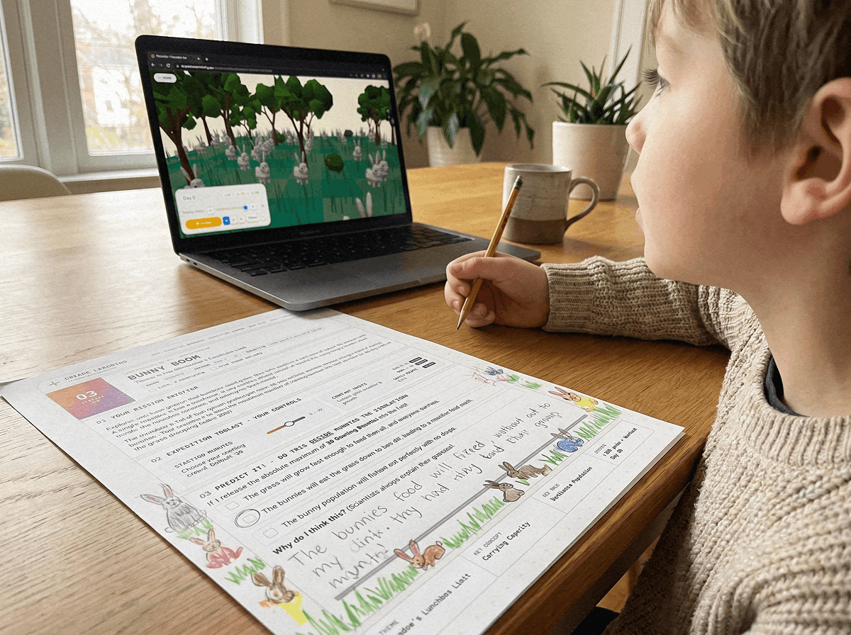
The Praxos 3D Predator-Prey Simulation transforms abstract differential equations into living biological reality. Students introduce wolves into a rabbit meadow and immediately see the delayed feedback loop unfold in real-time 3D and on live population telemetry charts.
By manipulating starting pack sizes, grazing rates, and environmental conditions, students discover the three classic regimes of population biology: stable oscillation, damped equilibrium, and catastrophic extinction collapse.
Jump into Level 4 ("The Gray Shadow") to balance wolves and rabbits in real-time 3D with live population line charts. Zero downloads, zero logins, and 100% free.
LAUNCH SIMULATOR NOWThe Three Dynamic Regimes in the Simulation
When students experiment in Level 4 and Level 5, their simulation runs generate three distinct mathematical outcomes based on their starting parameters:
1. Stable Limit Cycle: Predators and prey oscillate continuously without either species going extinct. Prey boom first, predators follow 15 to 20 simulation ticks later, and both species remain within sustainable bounds.
2. Overexploitation Crash: Introducing too many predators initially drives prey to zero within 30 ticks. Without food, predators starve to zero shortly after, resulting in total dual-species extinction.
3. Carrying Capacity Overshoot: If predators are removed entirely, prey multiply exponentially until all grassland vegetation is stripped, triggering a severe starvation collapse.
| Dynamic Regime | Starting Conditions | Prey Trend | Predator Trend | Ecosystem Outcome |
|---|---|---|---|---|
| Target EquilibriumStable Oscillation | Balanced starting ratio (1 wolf : 15 rabbits) | Cyclic waves (20-60 range) | Delayed cyclic waves (2-8 range) | Perpetual multi-generation balance |
| Prey Extinction Cascade | Predator overstocking (8+ wolves : 15 rabbits) | Steep drop to 0 within 25 ticks | Brief surge, then crash to 0 | Complete trophic collapse |
| Herbivore Boom & Crash | Zero predators (0 wolves : 25 rabbits) | Exponential surge to 80+, then crash | Absent (0) | Grass depletion, soil erosion |
Next Generation Science Standards (NGSS) Alignment
This free predator-prey simulation directly addresses NGSS performance expectations across middle school and early high school life sciences:
MS-LS2-2: Construct an explanation that predicts patterns of interactions among organisms across multiple ecosystems. Students analyze how predator hunting pressure regulates herbivore density and plant cover.
MS-LS2-4: Construct an argument supported by empirical evidence that changes to physical or biological components of an ecosystem affect populations.
HS-LS2-2: Use mathematical representations to support and revise explanations based on evidence about factors affecting biodiversity and populations in ecosystems of different scales.
Common Core Mathematical Practice MP.4: Model with mathematics. Students collect discrete population tick counts and plot coordinate curves to measure wave periods and amplitude shifts.
45-Minute Classroom Lab Plan: The Lotka-Volterra Graphing Lab
Here is a structured, zero-prep lesson plan designed for a standard 45-minute science block:
Pre-Lab Prediction & Variable Setup (10 Minutes)
Distribute the printable 24-page science journal. Students write a hypothesis predicting what happens to rabbit population peaks when 2 vs. 6 wolves are introduced.
Interactive 3D Simulation Trials (20 Minutes)
Students launch Level 4 on their Chromebooks or tablets. They run three 150-tick trials, pausing at ticks 25, 50, 75, 100, 125, and 150 to record species counts in their journal data table.
Coordinate Graphing & Lag Time Calculation (10 Minutes)
Using the recorded data table, students plot two colored curves (green for rabbits, gray for wolves) on the grid and calculate the exact time lag between the two peaks.
CER Scientific Synthesis (5 Minutes)
Students write a Claim-Evidence-Reasoning statement explaining why predators act as stabilizing feedback controllers in grassland biomes.
Chromebook Compatibility & Zero-Friction Classroom Access
Praxos Learning is built from the ground up for modern school environments:
Browser Compatibility: Tested on Google Chrome 90+, Microsoft Edge 89+, Apple Safari 14+, and Mozilla Firefox 85+.
Chromebook Ready: Lightweight WebGL 3D rendering optimized for standard 2GB RAM student Chromebooks and school tablets.
Zero IT Friction: Runs 100% in-browser with no installations, extensions, or administrative approval required.
Student Privacy: Zero student personal identifiable information (PII) is collected. No student accounts or passwords needed.
Frequently Asked Questions From Science Teachers
Answers to common questions about using the predator-prey simulation in middle school and high school classrooms.
What is the simplest way to explain Lotka-Volterra oscillations to middle schoolers?
Can AP Biology or Environmental Science students use this simulation for mathematical modeling?
Does this simulation require student email addresses or logins?
How many students can run the simulation at the same time in one room?
Is the simulation free for public schools and homeschool families?
Free Supporting Science & Population Ecology Resources
Deepen your ecology and population dynamics units with these free interactive resources:
The trophic cascade simulation online explores apex predator wolf reintroduction and whole-ecosystem restoration.
The free carrying capacity simulation game walks students through herbivore overpopulation and habitat resource limits.
The free food web simulator for kids enables students to construct multi-tiered producer-consumer-decomposer energy chains.
The prairie ecosystem simulation models native North American grassland energy balance in interactive 3D.
Get the complete printable PDF lab packet featuring coordinate graphing grids, population tick observation tables, and CER written prompts. Black-and-white printer friendly.
GET FREE LAB JOURNALFree 24-Page Predator-Prey & Ecology Lab Journal (PDF)
Printable coordinate graphing sheets, population data tables for 150-tick simulation runs, and Claim-Evidence-Reasoning (CER) prompts. Formatted for black-and-white classroom printing.